IntroductionHey guys, so this is a shorter, more informal post about a basic mathematical topic. Before we start, I made a pdf of this blog post using LaTeX. If you wish, you can read this exact post on the pdf here. In the past day, one of my friends asked me for help on an interesting calculus problem shown below: If $f$ and $g$ are inverse functions, then: $$\int_{a}^{b} f(x) dx = bf(b) - af(a) - \int_{f(a)}^{f(b)} g(y) dy$$ At first, when I looked at it, I thought the problem itself was incredibly interesting since it did not seem at all intuitive. Anyway, I worked on it for about ten minutes, trying everything from $u$-sub, to the mean-value-theorem to the fundamental theorem of calculus looking for some sort of solution. After about 15 minutes, at last I realized, it was the bane of all calculus, integration by parts! The reason I say integration by parts is the ``bane of calculus'' is because its hard to visualize integration by parts, and the theorem itself seems to come out of no where. The same is true for the solution to this problem which I will now present. Proof Using Integration By Parts To prove this theorem, consider $u = f(x)$ and $dv = 1$ (the function 1). Therefore $v = x$. Then, performing integration by parts on $u$ and $dv$ we have the following: $$\int_{a}^{b} f(x) dx = uv - \int vdu = xf(x)|_a^{b} - \int_{a}^{b} xf'(x) dx$$ Now, we use a $u$-sub, except my $u$ will be $y$. So we have $y = f(x)$, then $dy = f'(x) dx$. Here is the punchline: Since $g(f(x)) = x$, we see that $g(y) = x$. So we can finish the substitution of the last integral as $\int_{f(a)}^{f(b)} g(y) dy$, so we have in total: $$\int_{a}^{b} f(x) dx = bf(b) - af(a) - \int_{f(a)}^{f(b)} g(y) dy$$ A Nagging FeelingSo yeah, I finished the proof and gave my friend hints until she was able to figure it out for herself, and that should have been the end of it right?. Well, I had a nagging feeling that something else was going on. It did not seem so likely that integration by parts out of all things could solve something that looked so elegant and bizarre. I figured there had to be a visual proof that relates the integral of a function to the integral of its inverse right!? The next day, I was in the shower, and I was lucky to have a window next to me. So I steamed up the shower and started drawing on the window creating picture to help me understand what was going on. It was here I had an epiphany which I want to share with you guys. Proof Without Words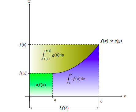 From here we see that $$\int_{a}^{b} f(x) dx = bf(b) - af(a) - \int_{f(a)}^{f(b)} g(y) dy$$ ConclusionThe above proof is not only simple, but beautiful and it avoids the non-visual pitfalls of using integration by parts. Consequently, this problem illustrates an important phenomena in mathematics: visualization. Visualization is important because it helps connect ideas within mathematics. As humans, we learn through visual effects, and not through formulas. Writing formulas as visual ideas can not only help us strengthen our understanding of the formulas, but also help us explore deeper ideas. The theorem itself relates the notion of inverses to their integrals, but the visualization shows us how the graphical notion of inverses allows for this theorem to be true. Additionally, this visualization strengthens the notion of integration with the notion of area, since by relating the two terms in this way, we can get more familiar with how integrals of inverse functions operate. Finally, the visualization avoids the pitfalls of formulaic mathematics such as the 'integration by parts formula' and demonstrates a deeper, and frankly cooler idea behind the formula.
1 Comment
Machine Learning OverviewOkay, so what is machine learning. Well, if you think about how humans learn, the process essentially involves repeated action, and using each trial of action to further your ability and enhance your ability to do a task. In other words, its about practice and training. Machine learning is similar. There are two types of machine learning, supervised learning and unsupervised learning. Unsupervised learning algorithm are fed a bunch of data and designed to create, enhance, or find features within the data that are otherwise hard to detect. For instance, let us say you are trying to group houses into categories given the number of rooms, the size of a house, and the number of bathrooms as variables $x$, $y$ and $z$. An unsupervised learning algorithm might learn that there exists a natural boundary between small, medium, and large sized houses. An example is shown below: 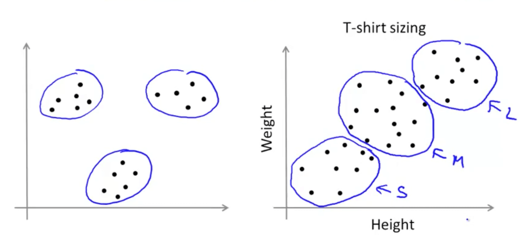 In contrast a supervised learning algorithm focuses mainly on drawing inferences on labeled data. For instance, this time, the goal is not to group houses into random categories, rather it is to learn their price. In other words, the objective of the algorithm is to use data about the house (sq. ft, area, rooms, bathrooms) to generate an estimate of the house's price. It does so by training on labeled data (or a sample of houses from which the all the information is known). Today, we are going to talk about Logistic Regression, one of the fundamental supervised machine learning algorithms in use today. We will also discuss Logistic Regression in the context of the Titanic Kaggle competition, a project that I recently completed. For those of you who did not know, Kaggle is a website that hosts a bunch of machine learning competitions that, if won, can result in large prizes (over 100K). For more resources on logistic regression, please check out Andrew Ng's course here. Additionally, I have written the code up for this blog post here at my Github if you wish to view it early. Logistic RegressionLogistic regression is a basic binary classification algorithm that takes in input data and outputs either 0 or 1. The data set we are using is the Titanic dataset which contains information on each of the passengers on the Titanic and whether or not they survived or died. To create this binary classifier, we use the sigmoid function $\sigma(\mathbf{x})$ defined as: $$\sigma(\mathbf{x}) = \frac{1}{1 + e^{-\mathbf{\theta}^T\mathbf{x}}}$$ 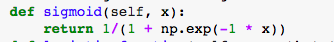 The function looks like the plot below:  The nice thing about this function is that it will take its input and scale it either to 0 if the input is very negative or 1 if the input is very positive. The input to this function, in our case is $\mathbf{\theta}^T\mathbf{x}$ where $\mathbf{x}$ is the vector that defines our data, and $\mathbf{\theta}$ is a vector of weights. We note that $\mathbf{\theta}^T\mathbf{x}$ is the same as taking the dot product between $\mathbf{\theta}$ and $\mathbf{x}$. (Note: Just because we use this function as a classifier does not mean that it will work perfectly. In fact, we will see that a trained classifier will not necessarily perform the best in this situation. Other models/functions can be tried but we will get to those later). Now that we have our classifier, let us get to the actual learning TrainingThere are two stages to any supervised machine learning algorithm: training and testing. Training is the process by which the computer uses labeled data (or training data) to fine tune the parameters of the algorithm. This is done by a process known as gradient descent. But before we get there, we need a way to define how well our algorithm is doing. We will use a metric defined as a part of information theory known as cross-entropy. There are other metrics we could use such as $L_1$ or $L_2$ (mean-squared error) but we will stick with cross-entropy since it makes gradient descent easier. So for each training point $i$ in our set we have a vector $\mathbf{x}$ of input data and an output $y$ that is either 0 or 1. The classifier will predict a value $\hat{y}$ that we want to be as close to $y$ as possible. The cross-entropy error $h(\mathbf{\theta})$ of a single data point is simply $-ylog(\hat{y}) - (1-y)log(1-\hat{y})$. The negative signs are there to change all of the logs into positive values (since $log(x) < 0$ if $0 < x < 1$). To find the total cross entropy error, we simply average over all training points. Now, we want to find the values of $\mathbf{\theta}$ such that our cross-entropy error is at a minimum. We can imagine that the function $h(\mathbf{\theta})$ is a function in some dimensional face perhaps like the one below:  For reasons I will not explain, the logistic function is convex meaning that it only has one minimum (this has to do with the choice of cross entropy and the sigmoid function). What this means is that we by simply following the gradient of the function (the direction of maximum decrease) we can get to the minimum. For instance, imagine yourself, on one of the large hills (but not at the top). Then, you can feel the slope going in some direction up or down. From there you can run down the hill into the valley (in blue), and you have reached the minimum. The algorithm does the same thing by measuring the gradient of the function at the point. The gradient, is a term in multi-variable calculus that is essentially a derivative except as a vector. Once we find the gradient, we can take a step in that direction, constantly moving until we reach the minimum. Calculating the GradientWarning: The following section is very technical so, first let us define some notation. Let our set of training data be a $S$ of pairs $(\mathbf{x}, y)$ where each pair has a vector of input data and its classification $y$. The set $S$ will have $m$ training examples. Each vector $\mathbf{x} \in S$ has $n$ components. We let $\mathbf{x}^{(j)}$ mean the $j$'th training example. Plugging into the cross entropy function, we have: $$-\frac{1}{m}\sum_{j = 0}^{m} (1 - y^{(j)})\log(1 - \sigma(\mathbf{x^{(j)}})) + y^{(j)}\log(\sigma(\mathbf{x^{(j)}}))$$ Okay, now let us compute the derivative of the sigmoid function, since we will need to employ the sigmoid function in our computation. $$\frac{d}{d x} \sigma(x) = \frac{d}{dx} \frac{1}{1 + e^{-x}} = \theta_i \cdot \frac{e^{-x}}{(1 - e^{-x})^2}$$. Now separate the last fraction into $\frac{1 - e^{-x}}{(1 - e^{-x})^2} - \frac{1}{(1 - e^{-x})^2} = \frac{1}{1 - e^{-x}} - \frac{1}{(1 - e^{-x})^2}$. This is equal to our final solution $(1 -\frac{1}{1 + e^{-x}})\frac{1}{1 + e^{-x}} = (1 - \sigma(x)) \sigma(x)$ By chain rule, then $\frac{\partial}{\partial \theta_i} \sigma(\mathbf{x}) = \sigma(\mathbf{x})(1 - \sigma(\mathbf{x})) \cdot \frac{\partial \mathbf{\theta}^T \mathbf{x}}{\partial \theta_i} = x_i\sigma(\mathbf{x})(1 - \sigma(\mathbf{x}))$. Now, we wish to calculate the derivative cross entropy function itself. We first take the derivative of the cross entropy function with respect to $\hat{y}$ since that is our sigmoid function. We obtain: $$-\frac{1}{m}\sum_{j = 0}^{m} (1 - y^{(j)})\frac{-\hat{y}'}{1 - \hat{y}} + y^{(j)}\frac{\hat{y}'}{\hat{y}}$$ Since, $\hat{y}' = \hat{y}(1 - \hat{y})$, we have $$-\frac{1}{m}\sum_{j = 0}^{m} -(1 - y^ {(j)}) \hat{y} + y^{(j)} (1 - \hat{y}) = -\sum_{j = 0}^{m} (y^{(j)} - \hat{y})$$. So far, this has been the derivative with respect to $\hat{y}$. To ge the derivative with respect to the thetas we have to use chain rule, specifically we let $\hat{y} = \sigma(\mathbf{x^{(j)}})$. Using chain rule we have: $$\frac{\partial J}{\partial \theta_i} = -\frac{1}{m}\sum_{j = 0}^{m} (y^{(j)} - \sigma(\mathbf{x^{(j)}})) \cdot x_i^{(j)} = \frac{1}{m}\sum_{j = 0}^{m} (\sigma(\mathbf{x^{(j)}}) - y^{(j)}) \cdot x_i^{(j)} $$ RegularizationThe last thing I want to talk about is regularization. This is the part of the algorithm which prevents overfitting. Overfitting essentially means fitting the training data too well, so that the algorithm itself is not generalizable. Testing data will not be the same as the training data, or necessarily follow the same exact patterns. Therefore, we employ a simple mathematical trick to keep all the theta's small. That way there is no wild variation. To do this, we simply sum over the squares of each variable parameter (and scale it down by a factor of 2m) and add this to our cost function. This way, when we minimize the cost function, we are also adding a tradeoff between our function and our regularization. It looks something like this: $$\frac{-1}{m}\sum_{j = 0}^{m} (1 - y^{(j)})\log(1 - \sigma(\mathbf{x^{(j)}})) + y^{(j)}\log(\sigma(\mathbf{x^{(j)}})) + \frac{\lambda}{2m}\sum_{\theta_i}^{n} (\theta_i)^2$$ Where $\lambda$ is a regularization parameter that we set manually. Consequently, to each derivative term, we simply add the term $\frac{\lambda}{m} \cdot \theta_i$ to our gradient function. Writing CodeNow, that we have figured out all the math, it is time to write it up. The first thing we need to do is scale our data and append a bias term to it. Essentially, this amounts to adding a $1$ to the end of every data point since when taking the dot product of $\mathbf{x}$ and $\mathbf{\theta}$ the $1$ at the end will multiply with the final theta in $\mathbf{\theta}$ to produce a bias. From there we implement a method called train which takes in data and trains it. If done correctly, the algorithm should look something like the code located here (when you get to the link, scroll down until you get to the Logistic Regression class). A final, practical use for writing any machine learning algorithm is checking your math. This is done through numerical gradient checking. Basically, we estimate $\frac{\partial J}{\partial \theta_i}$ through the usual limit definition of a derivative. In other words, we compute: $$\frac{J(\theta + \epsilon) - J(\theta)}{\epsilon}$$ For each $\theta_i$ and check it with our math. The reason we don't do this instead, is because it becomes computationally expensive very quickly. With code, it looks like the function below: 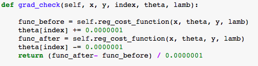 TestingFinally, we have completed the training for our first machine learning algorithm. Now that we are done with that, we can move on to testing! Once we train our algorithm on the data, testing is easy. We simply plug in the data we wish to classify as new values of $\mathbf{x}$ and see what the algorithm outputs. If done correctly, it should look like below: 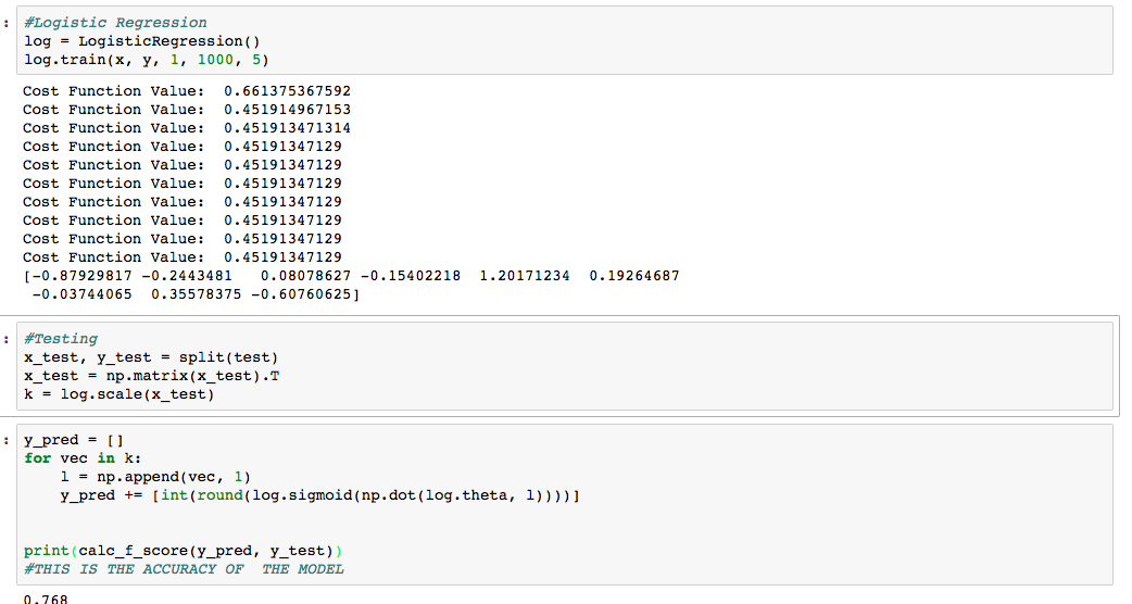 Wait what only a 0.768 F-score (85% accuracy)? (For details on the F-score metric go here). Well, the important thing to understand with Logistic Regression is that its not perfect. The algorithm itself may be too simple to try and understand the complexity of the data. Regardless, the algorithm implemented is not a bad one, but it can be expanded upon. In fact, logistic regression is one of the key parts of a neural network, something that will be talked about later! ConclusionYeah, this post was a long one, but to whoever is out there reading this, thank you for doing so. I want to do these sort of machine learning algorithm of the day thing once every two weeks or so, but we will see how it goes. Comment and let me know how I can improve, I am new to this whole blog thing after all, and I am learning along side all of you!
IntroductionMany of you have probably heard the advances that a machine learning algorithm, AlphaGo, has achieved in beating the top player of Go in the game. Basically, researchers designed an algorithm consisting of a neural network that was able to play the game Go better than the top Go player in the entire world, and is considered a massive feat in machine learning. Now researchers have done the same thing in Chess using a program known as AlphaZero. As a chess enthusiast myself, I was particularly interested in how the algorithm worked, since on first hearing about the accomplishment, I was appalled. To put this into perspective, researchers designed a deep neural network consisting of an general reinforcement learning algorithm. This means that the computer was only fed the rules of the game of Chess before training, with no other knowledge of opening theory, endgame techniques, etc. And with little modification, this algorithm was extended to Shogi and Go, beating the top engines in both games, including AlphaGo. With regards to Chess, AlphaZero beat Chess Engine Stockfish in a 100 game match 28 - 72 - 0, meaning it won 28, drew 72, and lost 0 chess games against Stockfish, a chess engine known to have already beaten the top chess players. 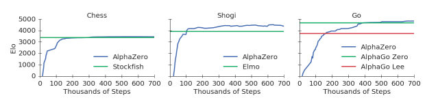 Additionally, while Stockfish took years to perfect, incorporating opening theory, endgame techniques, and quantifying small differences in positions, AlphaZero only trained for four hours before destroying Stockfish. In fact, AlphaZero need only calculate 80,000 board positions per second as compared to Stockfish's 7 million positions per second. If you wish to check out some of the games or read about the algorithm, read this paper (currently in development) by the Google DeepMind Team. Additionally, you can check out numerous articles on Chess.com or look at the Youtube channel ChessNetwork (my personal favorite) for an analysis on some of the games. I will leave a video of one analysis below. The AlgorithmOkay, so now that the introduction is out of the way, let us actually dive into the algorithm. My sources come mainly from this paper (linked above as well) as well as this infographic on AlphaZero Go (NOT AlphaZero, but similar), which you may find useful in explaining the problem. The algorithm in general is made up of two things, a deep neural network (DNN) and Monte-Carlo Tree Search (MCTS). We will first describe the Deep Neural Network and then explain its usage in Monte-Carlo Tree Search. Deep Neural Network In this section, I am only going to describe how the network is used in the algorithm, rather than the linear algebra that goes into it. If you wish to learn a bit more about that, watch these videos by 3Blue1Brown or read this blog post. I will also probably have my own blog post on how they work sooner or later. In regards to the structure, I cannot exactly say what the neural network structure is, since the paper does not specify what it is exactly, however, the infographic linked to above specifies the structure used for the AlphaGo Zero algorithm used in a previous Deep Mind project. The paper compares the two algorithms directly, and does not specify a difference in neural network structure, therefore I will assume that the structures are similar, if not the same. For now, assume the neural network is simply a function $f$ that starts out with some arbitrary parameters $\theta$, that once trained on some training data, can emulate a reasonable function that acts similar to the training data. So in general, the Deep Neural Network that is used in this program is assigned to do one thing: take in a board state (an arbitrary chess position), $s$, and output move probabilities $p$ (the probability that this next move is 'good') as well as the expected outcome of the current move $v$ (The expected value that this move will lead to a win). So for instance, if the board state is the move d4, then the neural network would produce probabilities for d5, Nf3, etc, and would give the expected outcome of the move d4, which will be some number between -1 and 1. (-1 signifying a loss and 1 signifying a win) So normally, after designing such an algorithm, one would expect to give it some data in order to optimize the parameters used in the neural net. However, since this is a general reinforcement learning algorithm, the neural net cannot be given any outside data except for the rules of the game. So, how does the network get its data? Through self play and Monte-Carlo Tree Search. Monte-Carlo Tree SearchMonte-Carlo Tree search is an algorithm that basically helps hone in on what moves are better than others in regards to the chess world. The algorithm starts with a tree with a single node representing the board state $s$, which for our purposes means that the algorithm starts with the opening position in Chess. Each node in this tree is representative of a board states, with states being connected by edges only if you can move from one state to the other. Additionally each node has four values that go with it, $N$, $W$, $Q$ and $P$, where $N$ is the number of times the node is visited (originally set to 0), $W$ is the total value of that node (originally set to 0), $Q$ is the average value of the node (set to $W/ N$) and P is the probability assigned to the node by the Deep Neural Network (set to 1 since its the opening position). Starting from the single node, the current board state is fed into the Neural Network which outputs two things, the probability of moving to the next stage ($p$) and the value of the current state, $v$. Once this is done, it creates a new layer of nodes (in this case nodes corresponding to all possible opening moves such as e4, d4, c4, etc..). When initializing these nodes, we set the probability $P$ equal to the probability assigned by the neural network. However, this is just the first step, in the second and general steps there are some more complexities. 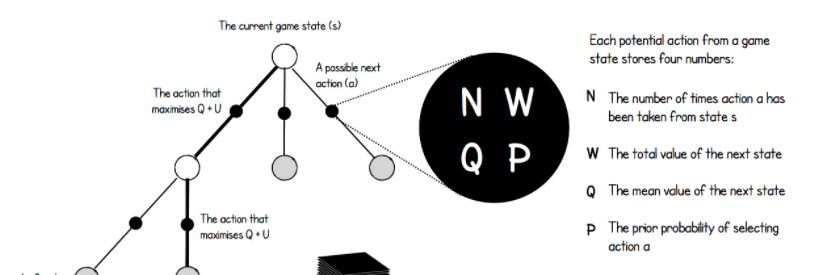 The second step (or any general step) repeats the computation, except it starts at the current board state (in this case the starting position) and proceeds down the tree until it reaches a leaf node by maximizing $Q + U(N, P)$ where $U$ is some function (not specified in the paper/infographic) involving $N$ and $P$. I will get back to the reason behind this decision later. Once it has gotten to the the leaf node, it feeds the board state $s$ it is currently at into the neural net, which outputs probabilities for another layer of nodes as well as a value $v$. Once again a new layer of nodes is created corresponding to the board states of all possible moves after the current move. This time, however, every board-state node that preceded $s$ has its $N$, $Q$ and $W$ updated as follows: $N = N + 1$, $W = W + v$ and $Q = W / N$. These steps are repeated some arbitrary number of times (for AlphaZero Go it was 1600). Then once this has happened, the tree is very expansive and filled with a lot of data. AlphaZero at this point chooses a move based on the probabilities $\pi$ corresponding to the $N$ values of each move that comes after the original state. So lets say the state was at the starting position, and lets say the only moves that had $N > 0$ were a4, e4, and d4 with $N_{\text{a4}} = 300$, $N_{\text{e4}} = 600$, and $N_{\text{d4}} = 100$. In this case $\pi$ would be $(0.3, 0.6, 0.1)$ and I would choose a4 with a 30% probability, e4 with a 60% probability and d4 with a 10% probability. This is regardless of whatever else is in the tree. The point is that after a move is chosen, the tree is not discarded, rather the root of the tree now moves down and becomes whatever board state is chosen. Additionally after the move is chosen, the board state of the game is recorded along with the probability vector $\pi$. This represents one data point, and will be used to train the DNN later. Now, after the move is chosen, the same cycle of 1600 simulations is repeated again, generating more and more of the tree. This is basically done until the game finishes, either in checkmate or a draw (based on the rules of Chess). Once this is done, each of the board state data points are updated to include the result $z$ of the game (either -1, 0 or 1). Now getting back to the earlier point of why $Q + U(N, P)$ is used as the function to decide how to move. The reason for this is that at first, $U$ dominates forcing more exploration among the nodes, so breadth is key, whereas later in the game $Q$ dominates, forcing the program to follow a more precise (not-breadth) approach. This allows both for versatility in the opening, and precision in the middle/end games. And there you have it, this is how AlphaZero plays one game against itself. If it were to play against an opponent, the only difference would be that instead of choosing the next move probabilistically, it would choose the move deterministically (always choose the move with the highest probability in $\pi$). Training the Deep Neural NetworkTo train the neural network, first the algorithm plays some number of games against itself (not specified). After doing so, it has many data-points consisting of a board state (s), a probability vector $\pi$ and an outcome $z$. It uses these values to train itself trying to minimize the loss function $(z- v)^2 + \pi^{T}log(p) + c|\theta|^2$ where the first expression is mean-squared error, the second expression is cross entropy, and the third expression is regularization (combatting overfitting). To train, the network uses batch-gradient descent, which basically means it takes a number of samples (4096 to be exact) and computes the gradient minimizing the loss function on just that data. It takes one step, throws out the data and chooses another 4096 data points from the space, and repeats some number of times. After this is all done, the network is trained and ready to go....play another set of matches against itself. This generates new data points, which are then used to retrain the neural network many times over. In order to measure its performance, the Chess ELO rating system is used, using Stockfish's actual rating as a baseline.  Comparing The Algorithm at the Beginning VS. the EndThe purpose of this section is to just compare what the algorithm looks like at the beginning of its development versus towards the end. The idea of this is to help you (the reader) and me better understand why such an algorithm was used in the first place. One of the questions I had when I first understood the algorithm was why it worked so well when at the beginning, the neural network would give such arbitrary results. Like, the probability vectors $\pi$ that are generated, are generated, ultimately, by the neural network itself with some slight adjustment. It is like feeding an untrained neural network random data and expecting it to pop up with some magical pattern. However, upon further reflection, I started to understand why there were two types of data collection. Not only were the probability vectors $\pi$ collected, but the outcome $z$ was also collected. This means at the beginning, the vectors $z$ were the main thing controlling the algorithm's development. The program was learning what lines constituted a win versus a loss. Later, towards the algorithm's matured development, the $p$'s would become more important, influencing nuanced chess play in the algorithm, since now single moves can either blunder the game or save it. Conclusion To conclude, AlphaZero is, in my opinion, one of the coolest programs ever invented on the internet. Whereas when AlphaGo beat the top Go player did not seem like such a big deal to me at the time, AlphaZero's domination against Stockfish has really shaped my view of what machine learning can do. I greatly enjoyed learning about the algorithm and writing it up for you guys to see. Thank you for reading!
|
AuthorMy Name is Ankit Agarwal. Check out the about me page for more information! Archives
February 2018
Categories
All
|
 RSS Feed
